Week 1 L3: Discrete time Signal Synthesis and capture
Contents
Introduction
Mathematical description of and MATLAB creation of discrete time
- delta function
- unit step
- unit exponential
- simple sinusoid


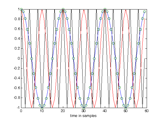
Sinusoid
figure(1)
N=60;   % Number of samlpes
n=0:N-1;  % Set up sample axis
x=cos(2*pi*.25*n)
plot(n,x,'k')
hold on
x=cos(2*pi*.1*n);
plot(n,x,'r')
x=cos(2*pi*.05*n);
plot(n,x,'b')
xlabel('time in samples')
plot(n,x,n,x,'o')
hold off
x =

  Columns 1 through 6

    1.0000    0.0000   -1.0000   -0.0000    1.0000    0.0000

  Columns 7 through 12

   -1.0000   -0.0000    1.0000    0.0000   -1.0000   -0.0000

  Columns 13 through 18

    1.0000   -0.0000   -1.0000   -0.0000    1.0000   -0.0000

  Columns 19 through 24

   -1.0000   -0.0000    1.0000   -0.0000   -1.0000   -0.0000

  Columns 25 through 30

    1.0000   -0.0000   -1.0000   -0.0000    1.0000   -0.0000

  Columns 31 through 36

   -1.0000   -0.0000    1.0000    0.0000   -1.0000   -0.0000

  Columns 37 through 42

    1.0000    0.0000   -1.0000   -0.0000    1.0000    0.0000

  Columns 43 through 48

   -1.0000   -0.0000    1.0000    0.0000   -1.0000    0.0000

  Columns 49 through 54

    1.0000    0.0000   -1.0000   -0.0000    1.0000    0.0000

  Columns 55 through 60

   -1.0000    0.0000    1.0000    0.0000   -1.0000   -0.0000
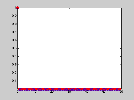
Delta function
figure(2)
delta=[1 zeros(1,N-1)];
stem(n,delta,'markersize',10,'markerfacecolor','r')
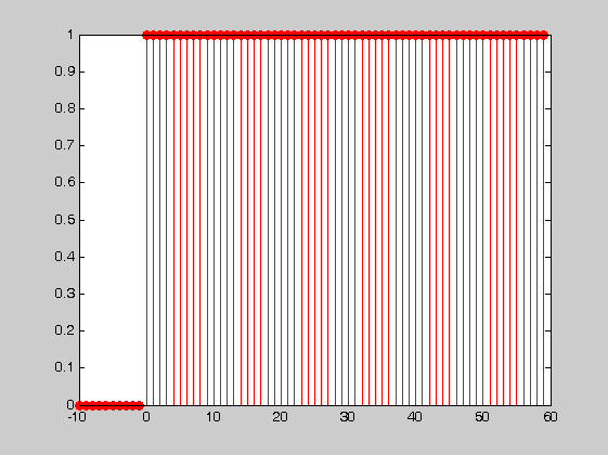
Step Function
figure(3)
% In this case we show some negative time
n=-10:N-1; % Set up the sample vector starting at n=-4 goint to n=N-1 (= 59)
unitstep=[zeros(1,10) ones(1,N)];
stem(n,unitstep,'r','markerfacecolor','r')
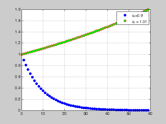
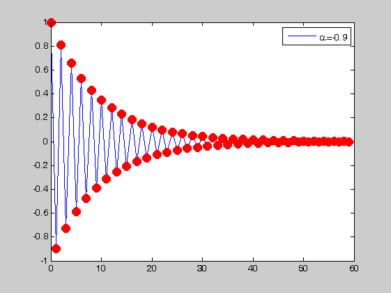
Unit exponential
figure(4)
n=0:N-1;
alpha=.9;
y=alpha.^n;
plot(n,y,'ob','markersize',6,'markerfacecolor','b')
hold on
grid on
alpha=1.01;
y=alpha.^n;
plot(n,y,'or','markersize',6,'markerfacecolor','g')
legend('\alpha=0.9','\alpha = 1.01')
figure(5)
alpha=-.9;
y=alpha.^n;
plot(n,y,'or','markersize',10,'markerfacecolor','r')
plot(n,y,n,y,'or','markersize',10,'markerfacecolor','r')
legend('\alpha=-0.9')