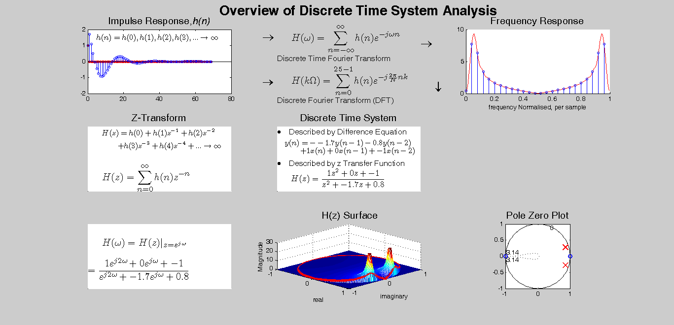
The Different views of a Discrete Time System
Richard Hayes, Dublin Institute of Technology
Contents
Introduction
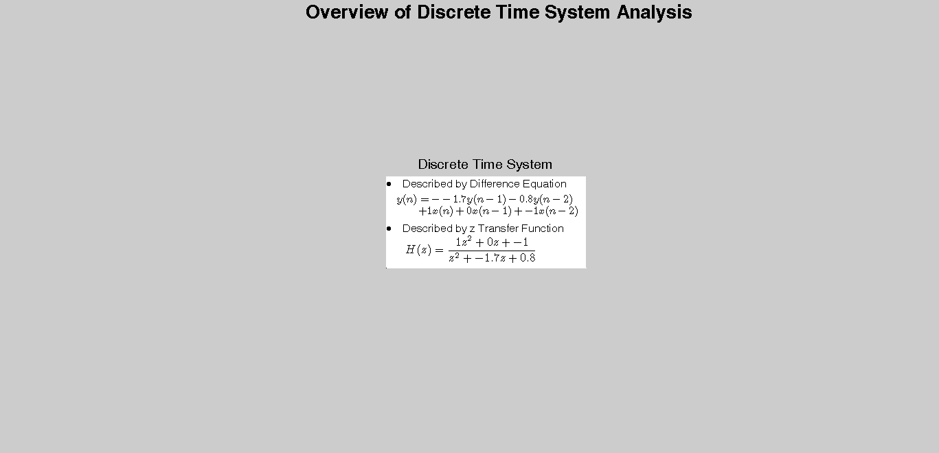
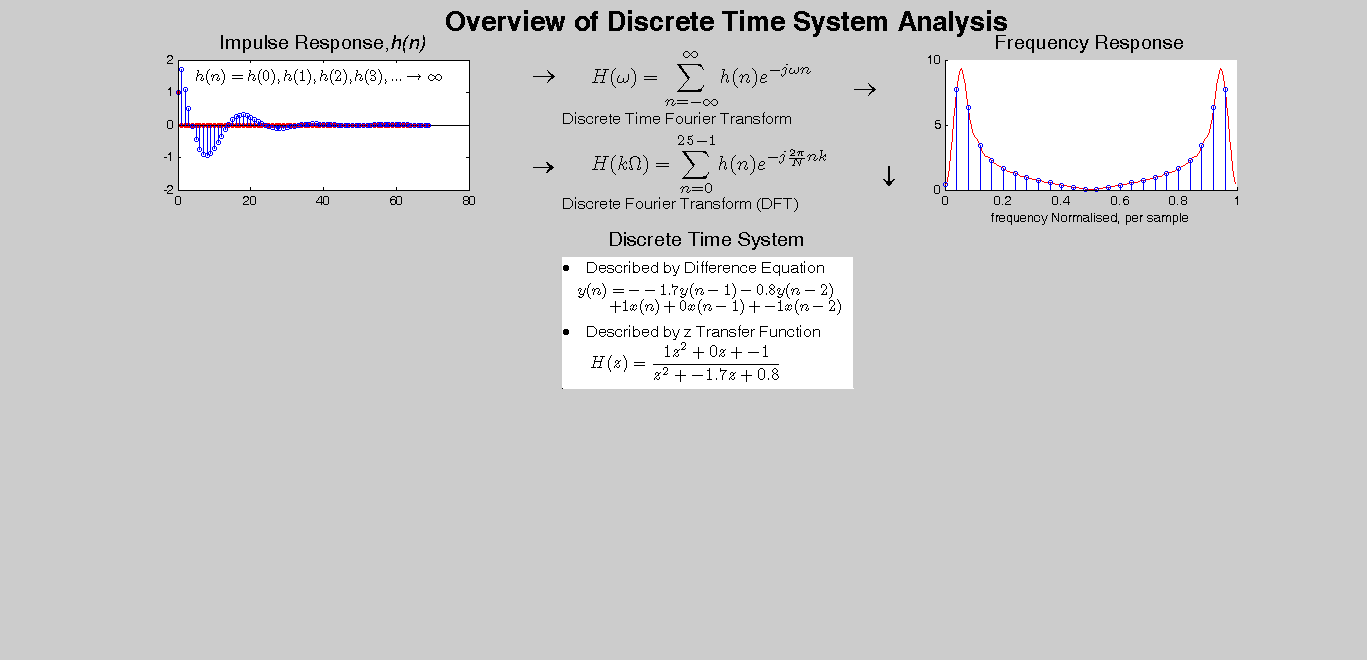
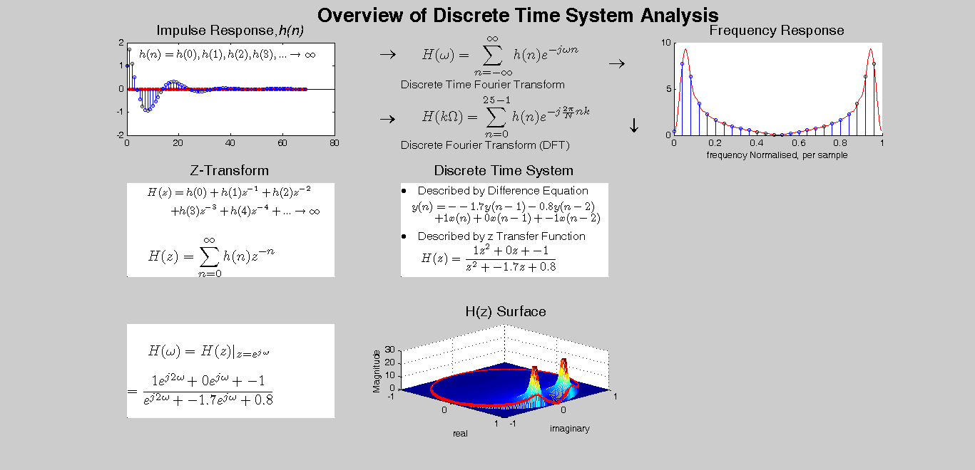
This note explores using MATLAB the fundamental relationships between the various views (mathematical descriptions ) of discrete time systems. Show Mathematical forms ofh(n) H(z) H(w) H(k)
- Difference Equation

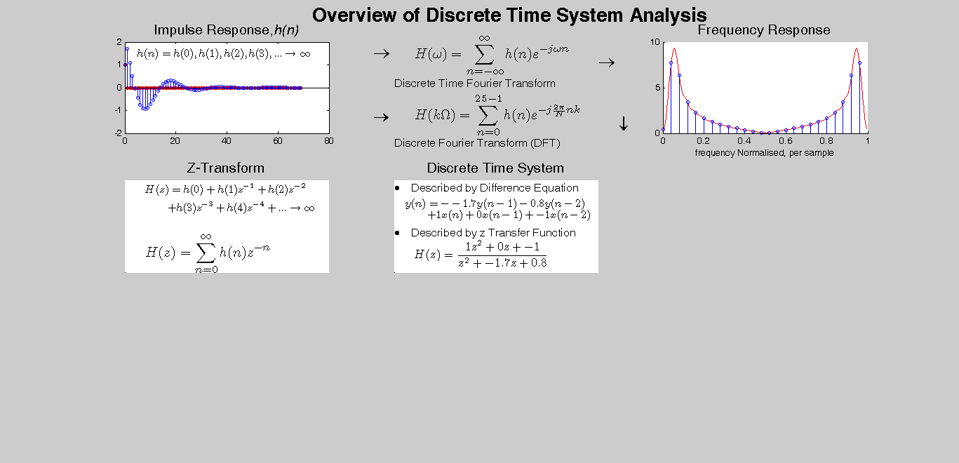
- Z-Transform
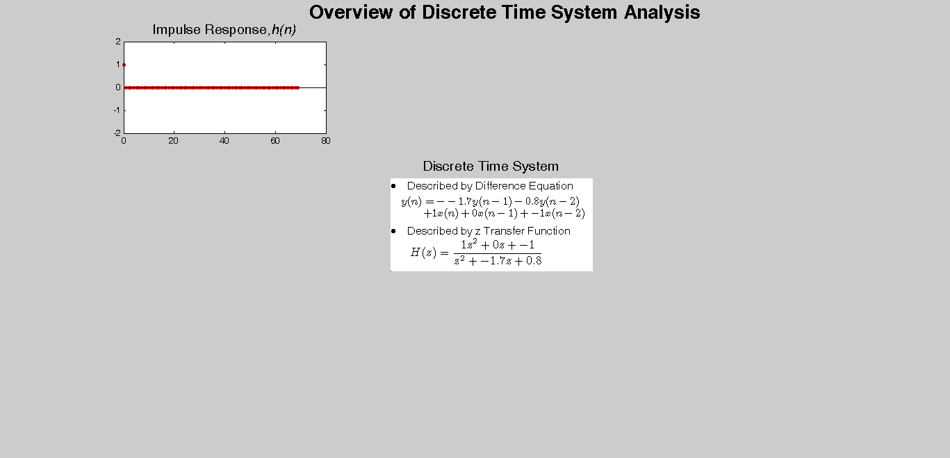
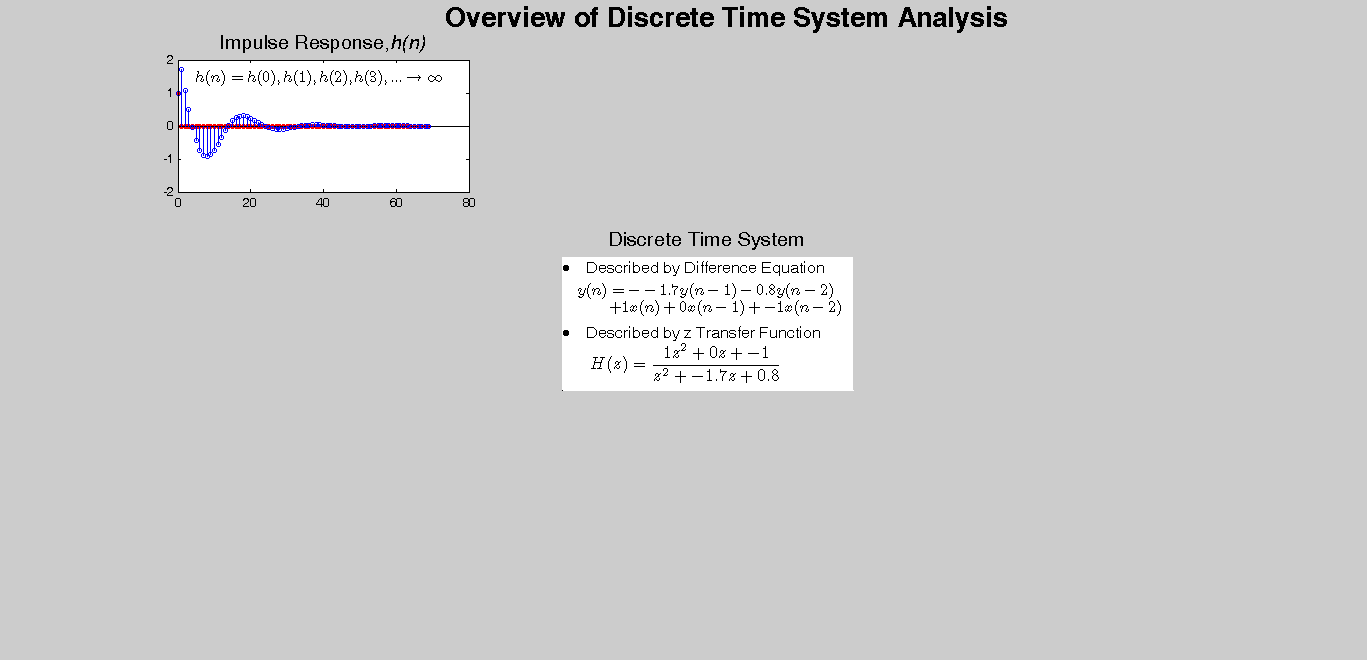
- Impulse Response

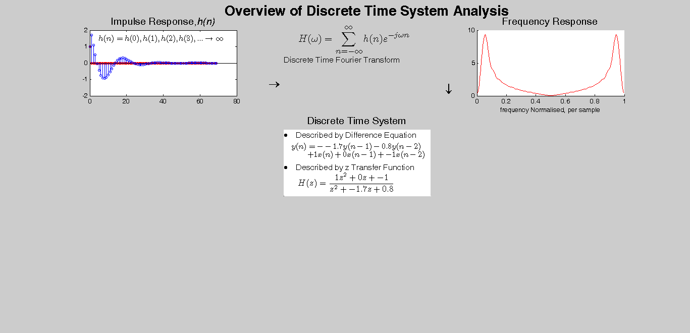
- Discrete Fourier Transform
- Fourier Transform
Difference Equation
b=[1 0 -1];a=[1 -1.4 .8];
figure(1)
clf
subplot(3,3,5)
DSP1OverviewWriteDE
Impulse response
subplot(3,3,1)
N=40;n=0:N-1;del=[1 zeros(1,N-1)];y=filter(b,a,del);h=y;
stem(n,del,'or','markersize',3,'markerfacecolor','r');ylim([-2 2]);hold on;%stem(n,del,'r')
title('Impulse Response,\ith(n)','fontsize',15);
pause
stem(n,y,'markersize',3);hold off
text('Interpreter','latex','String',['$$h(n)=h(0),h(1),h(2),h(3),...\rightarrow\infty$$'],...
        'Position',[5,1.5],'fontsize',12)
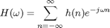
Fourier Transform (DTFT)
%N=25;
subplot(3,3,2)
 set(gca, 'visible', 'off');
text('Interpreter','latex','String',['$$H(\omega)=\sum_{n=-\infty}^{\infty}h(n)e^{-j\omega n}$$'],...
        'Position',[.1,.85],'fontsize',15)
text(0,.55,'Discrete Time Fourier Transform','fontsize',12,'fontweight','bold')
text(-.1,.2,'\rightarrow','FontSize',18,'FontWeight','bold');
text(1.1,.1,'\downarrow','FontSize',18,'FontWeight','bold')

% Take DFT of much larger N (= 250 below) to get closer to the Fourier
% Transform. This results in a continuous function of frequency, i.e. the
% frequency response H(w).
nfft=N*8;;n=0:N-1;del=[1 zeros(1,N-1)];y=filter(b,a,del);
H=fft(y,nfft);fax=0:1/nfft:(nfft-1)/nfft;
subplot(3,3,3);hold on;plot(fax,abs(H),'r');%hold off
%[H,w]=freqz(b,a,512,'whole');
title('Frequency Response','fontsize',15)
xlabel('frequency Normalised, per sample')
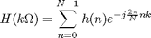
Discrete Fourier Transform (DFT)
subplot(3,3,2)
 set(gca, 'visible', 'off');
text('Interpreter','latex','String',['$$H(k\Omega)=\sum_{n=0}^{' num2str(N) '-1}h(n)e^{-j\frac{2\pi}{N} nk}$$'],...
        'Position',[.1,.2],'fontsize',15)
text(0,-.1,'Discrete Fourier Transform (DFT)','fontsize',12,'fontweight','bold')
text(-.1,.9,'\rightarrow','FontSize',18);text(1,.8,'\rightarrow','FontSize',18)
subplot(3,3,3)
n=0:N-1;del=[1 zeros(1,N-1)];y=filter(b,a,del);
H=fft(y);fax=0:1/N:(N-1)/N;stem(fax,abs(H),'markersize',3);
Z-transform
subplot(3,3,5)
%text(-.2,.5,'\leftarrow','FontSize',20,'FontWeight','bold');
%text(-.5,1.2,'\downarrow','FontSize',20,'FontWeight','bold');
subplot(3,3,4)
DSP1OverviewWriteZtransform
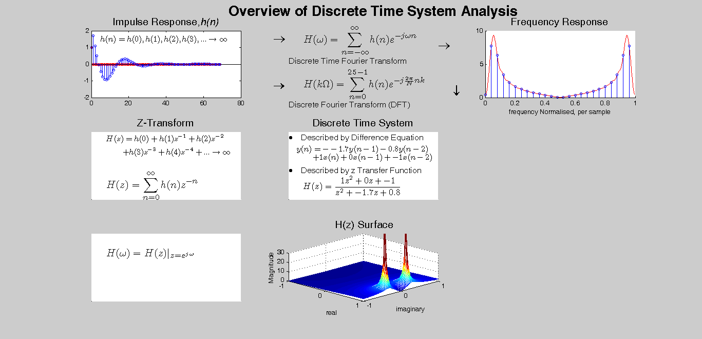
Z surface
subplot(3,3,8)
DSP1Overviewzsurface1

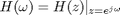
H(w) from the z-surface
subplot(3,3,7)
set(gca,'YTick',[])
set(gca,'YColor','w')
set(gca,'XTick',[])
set(gca,'XColor','w')
 text('Interpreter','latex','String',['$$H(\omega)=H(z)|_{z=e^{j\omega}}$$'],...
        'Position',[.1,.7],'fontsize',15)
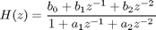
Transfer Function H(z) to H(w)
Let
text('Interpreter','latex','String',['$$=\frac{' num2str(b(1)) 'e^{j2\omega}+' num2str(b(2)) 'e^{j\omega}+' num2str(b(3)),...
    '}{e^{j2\omega}+' num2str(a(2)) 'e^{j\omega}+' num2str(a(3)) '}$$'],...
        'Position',[0,.3],'fontsize',15)
% text('Interpreter','latex','String',['$$=\frac{b_0e^{j2\omega}+b_1e^{j\omega}+b_2}{e^{j2\omega}+a_1e^{j\omega}+a_2}$$'],...
%         'Position',[.1,.2],'fontsize',15)%% Z surface
subplot(3,3,8)
DSP1Overviewzsurface2
Poles and Zeros
subplot(3,3,9)
ze=0.00001+j*0.00001;
axis('square')
zgrid(0,pi)
hold on
plot(roots(a),'xr','markersize',12,'linewidth',2)
plot(roots(b+ze),'o','linewidth',2)
hold off
title('Pole Zero Plot','fontsize',15)